


Table of contents
Recently, I'm reading the Positional Option Trading (2020) by Euan Sinclair. There is a section evaluating and comparing the performance of option structures such as straddle, strangle, butterfly, condor, etc. Euan performed the analysis with the simulated data, which I think is quite robust. Most importantly, this methodology may save a huge amount of costs on purchasing data, especially for options. Considering I'm just an unemployed college student with an empty pocket and lots of time, Building a simulator is very economically efficient.
In this article, I will implement a Class of Monte Carlo Simulator. Hopefully, there will be at least two types of simulations from (1) the normal distribution, or (2) the bootstrapped distribution.
Normal Distribution
Let's build the Class for normal distribution first.
For each simulation, there are three most important variables:
Drift (=mean of distribution): the trend of an asset
Volatility (=std of distribution): the fluctuation around the trend
Size: sample size
I also added two variables for more customizability:
Initial price: for parsing the series from percentage term to price term
Interval (day, week, month, quarter, or year): the frequency of returns
I then pass them to the set_normalParams() method. So, here is the constructor:
class MCSimulator():
  def __init__(self,initPrice=1,drift=0.08,volatility=0.20,size=252,interval='D'):
    self.set_normalParams(initPrice,drift,volatility,size,interval)
Note that, the drift and volatility are in annualized term for convention. (Default 8% annual drift, 20% annual volatility, 252 samples mimicking the one-year performance of the market index)
  def set_normalParams(self,initPrice,drift,volatility,size,interval):
    self.parse_interval(interval)

    self.initPrice = initPrice
    self.drift = drift/self.yearDivisor
    self.volatility = volatility/np.sqrt(self.yearDivisor)
    self.size = size

    self.print_charateristics()

  def parse_interval(self,interval):
    self.interval = {'D':1,'W':5,'M':21,'Q':63,'Y':252}[interval]
    self.yearDivisor = 252//self.interval
As the interval parameter is just a single character, we need to parse them to something meaningful.
parse_interval() parses the interval to the number of days. yearDivisor is just the fraction of a year to convert those annualized numbers. For example, weekly interval = 5 days so yearDivisor = 252//5 = approximately 50 weeks in a year. Thus you divide the yearly drift by 50 to get the weekly drift. This is exactly what I do for drift and volatility.
print_charateristics() is just for easier debugging. It prints out the instance variables. FYI:
  def print_charateristics(self):
    print(
f'''
initPrice = {self.initPrice}
drift = {self.drift}
volatility = {self.volatility}
size = {self.size}
interval = {self.interval}
yearDivisor = {self.yearDivisor}
'''
    )
Once we set the parameters for the distribution, we can go for the simulation, which is actually the easiest part to implement. We need one more parameter numPaths to specify how many times of simulation we want. Then, just put everything into the random number generator and let numpy do its job. returnSeries will store the DataFrame of return, each column represents one simulation, and each row represents a snapshot of every simulation at that time.
  def simulate_normal(self,numPaths=10000):
    self.numPaths = numPaths
    returnSeries = pd.DataFrame(np.random.normal(loc=self.drift,
                                                 scale=self.volatility,
                                                 size=(self.size,self.numPaths)
                                                 ))
    returnSeries.iloc[0,:] = 0
    self.priceSeries = self.initPrice * (1+returnSeries).cumprod()
    self.format_priceSeries()
    return self.priceSeries

  def format_priceSeries(self):
    self.priceSeries.reset_index(drop=True,inplace=True)
    self.priceSeries.index.name = 'Date'
    self.priceSeries.columns.name = 'Path'
The first row is set to be 0 return so that every simulation has the same starting point. Multiplying the cumulative return by the initial price give you the price series (the initial price is default 1, so the price series will be exactly the same as the cumulative return series). format_priceSeries() cleans up the DataFrame. Then, the priceSeries will be returned.
Let's see if it works.
sim = MCSimulator(initPrice=100,
                  drift=0.08,
                  volatility=0.20,
                  size=252,
                  interval='D')
sim.simulate_normal(numPaths=5)
Here's the result:
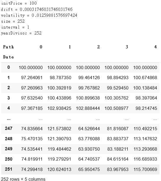
The expected runtime of 10000 simulations is 134 ms ± 18.9 ms per loop (mean ± std. dev. of 7 runs, 10 loops each). Not bad! Much cheaper than subscribing Bloomberg.
Bootstrapping
It's time for the bootstrapping. The framework is already established, so we only need some modifications.
First, we need an input of dataset. I assumed here the dataset to be a price series.
  def set_bootstrapPrice(self,priceData,initPrice=1,size=252,interval='D'):
    self.parse_interval(interval)

    self.initPrice = initPrice
    self.returnDist = priceData.pct_change(periods=self.interval)
    self.drift = self.returnDist.mean()
    self.volatility = self.returnDist.std()
    self.size = size

    self.print_charateristics()
Again, parse the interval, and set the initial price and size. One extra step is to transform the price series into percentage returns. The interval determines how many days we ignore for the calculation of return (maybe reducing noise or losing information, whatever). Then, calculate the drift, and the volatility in case the future me wants to use these parameters to simulate with normal distribution.
Done! We can modify the simulation method:
  def simulate_bootstrap(self,numPaths=10000):
    self.numPaths = numPaths
    returnSeries = pd.concat([self.returnDist.sample(n=self.size,
                                                       replace=True,
                                                       ignore_index=True) for _ in range(self.numPaths)],
                             axis=1,
                             keys=range(self.numPaths))
    returnSeries.iloc[0,:] = 0
    self.priceSeries = self.initPrice * (1+returnSeries).cumprod()
    self.format_priceSeries()
    return self.priceSeries
This time, the simulation is done by the sample method from pandas.Series. As it can only produce one simulation at a time, I used a for loop and pandas.concat to wrap them up. Everything else is copy and paste from the previous simulate_normal() method.
I tested it with the market index.
mkt = yf.download('^SPX')['Adj Close']

sim = MCSimulator()
sim.set_bootstrapPrice(mkt,initPrice=mkt[-1],size=252,interval='D')
sim.simulate_bootstrap(numPaths=5)
The initial price is set to be the latest price, so this simulator is forecasting the 5 possible paths of the next 252 days, please be ready to STONK ;)
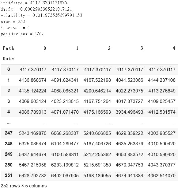
4 out of 5 simulations show an uptrend for the market. It's time to buy and get rich! (please don't)
Distribution
The simulation is not the main dish but the further analysis is. One thing we can do on the simulated price data is to backtest strategies on it. Or I just simply want to have a glance at the distribution characteristics. For example, I may want to know the distribution of the median given the bootstrapped distribution.
I can think of some metrics I can work with now:
Mean
Median
Std
Skewness
Kurtosis
10th quantile
90th quantile
Basically, they are just some numbers describing the distribution of the simulation. For example, the 10th quantile price may represent the expected hard times of the asset.
  def print_statsDist(self):
    stats = ['Mean','Median','Std','Skew','Kurt','10th','90th']
    statsDistDf = pd.DataFrame(columns=stats)

    dist = self.priceSeries

    statsDistDf.loc['Mean',stats] = self.cal_statsStats(dist.mean())
    statsDistDf.loc['Median',stats] = self.cal_statsStats(dist.median())
    statsDistDf.loc['Std',stats] = self.cal_statsStats(dist.std())
    statsDistDf.loc['Skew',stats] = self.cal_statsStats(dist.skew())
    statsDistDf.loc['Kurt',stats] = self.cal_statsStats(dist.kurt())
    statsDistDf.loc['10th',stats] = self.cal_statsStats(dist.quantile(q=0.10))
    statsDistDf.loc['90th',stats] = self.cal_statsStats(dist.quantile(q=0.90))

    print(statsDistDf)
cal_statsStats() may be confusing but it's just a method to calculate the distribution of the statistics across the simulations. To make my life easier, I will use the same metrics.
  def cal_statsStats(self,data):
    _mean = data.mean()
    _median = data.median()
    _std = data.std()
    _skew = data.skew()
    _kurt = data.kurt()
    _10th = data.quantile(q=0.10)
    _90th = data.quantile(q=0.90)
    return (_mean,_median,_std,_skew,_kurt,_10th,_90th)
The table returned looks like this:

I know it's confusing. Each row represents the distribution of that metric across simulations. For example, from every simulation, we can get the median of that simulation. Then, these medians from different simulations form a distribution of medians. The second row describes the characteristics of this distribution.
Further Development
For now, this simulator only generates many price series. One possible development is that I can feed some strategy rules into the simulator and it helps me to calculate the distribution of performance metrics such as Sharpe Ratio, or something like that. But it will not be as easy since these strategies themselves are not easy to generalize, like options strategy and trend-following strategy are totally different.