Rob Carver's Systematic Trading Framework 1. Choosing instruments

Inspired by Rob Carver's Systematic Trading (2015) and Advanced Futures Trading Strategies (2023), this series recorded how I demonstrate the trading / back-testing framework from Carver.
Plan
I will use Python and Jupyter Notebook for this project. 20-year daily data from Yahoo! Finance will be used for back-testing the performance.
# Libraries
import pandas as pd
import numpy as np
import matplotlib.pyplot as plt
import yfinance as yf
import itertools
Steps:
Choosing instruments
Trading rules and variations
Volatility targeting and position sizing
Systematic Trading (Rob Carver, 2015). Chapter 3, Framework
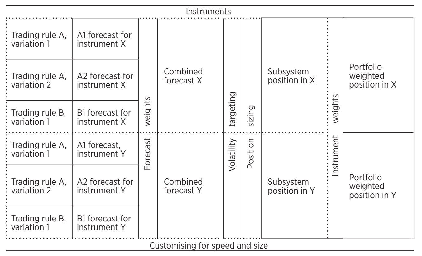
Step 1. Choosing instruments
Performance evaluation
To begin with, let's define an evaluation framework first. A well-defined framework allows us to compare the performance and examine the characteristics of different instruments / trading systems.
Performance metrics:
Annulized Daily Return
Annulized Daily Volatility
Sharpe Ratio
Skewness
Upper-tail Ratio
Lower-tail Ratio
Benchmark
For the choice of instruments, I am going for Ray Dalio's All Weather Portfolio. It's a portfolio aiming to achieve risk parity, meaning that all assets should have the same risks. For a passive investor, this provides steady returns even in hard times.
According to Lazy Portfolio ETF,
In the last 30 years, the Ray Dalio All Weather Portfolio obtained a 7.20% compound annual return, with a 7.21% standard deviation.
Assuming a zero risk-free rate (this is used for the whole project), this is a Sharpe Ratio of 1. I'm going to use a similar portfolio as the benchmark and to construct the system.
Ray Dalio All Weather Portfolio: ETF allocation and returns (Lazy Portfolio ETF, 2015)
| Weight (%) | Ticker | ETF Name | Investment Themes |
| 30.00 | VTI | Vanguard Total Stock Market | Equity, U.S., Large Cap |
| 40.00 | TLT | iShares 20+ Year Treasury Bond | Bond, U.S., Long-Term |
| 15.00 | IEI | iShares 3-7 Year Treasury Bond | Bond, U.S., Intermediate-Term |
| 7.50 | GLD | SPDR Gold Trust | Commodity, Gold |
| 7.50 | GSG | iShares S&P GSCI Commodity Indexed Trust | Commodity, Broad Diversified |
For simplicity, only VTI (equity), TLT (bond), and GLD (gold) will be used.
| Original weight (%) | Rescaled weight (%) | Ticker |
| 30.00 | 38.71 | VTI |
| 40.00 | 51.61 | TLT |
| 7.50 | 9.68 | GLD |
# Benchmark portfolio
symbols = ['VTI','TLT','GLD']
weights = [0.3871,0.5161,0.0968]

# Download 20-year daily data from YFinance
raw_data = yf.download(symbols,period='20y',interval='1d',prepost=False,repair=True)

# Indexing training/test data
train_index = raw_data.index[:len(raw_data)//2]
test_index = raw_data.index[len(raw_data)//2:]

# Use the adjusted close data only
prices = raw_data['Adj Close']
Compute the daily log returns for every instrument.
$$r_t = ln(p_t/p_{t-1}) = ln(p_t)-ln(p_{t-1})$$
def logReturns(prices,days=1):
  log_prices = np.log(prices)

  output = log_prices[::days].diff()
  return output

returns = logReturns(prices)
The weighted average return will be the return of the portfolio, assuming the portfolio re-balances the weight every day.
$$r_{BCHM,t} = \sum w_i \times r_{i,t}$$
# Daily return of benchmark
returns['BCHM'] = np.average(returns[symbols], weights=weights, axis=1)
Annualized return
Compute the annualized expected daily return.
$$Annualized Return=E(r) \times252$$
def annualizedReturn(returns,days=252):
  exp_ret = returns.mean()

  output = exp_ret*days
  return output
Annualized volatility
Compute the annualized daily volatility.
$$AnnualizedVolatility=\sigma \times \sqrt{252}$$
def annualizedVolatility(returns,days=252):
  vol = returns.std()

  output = vol*(days**0.5)
  return output
Sharpe Ratio
Compute the Sharpe Ratio (risk-free rate = 0).
$$SharpeRatio=\frac{AnnualizedReturn-r_f}{AnnualizedVolatility}$$
def sharpeRatio(returns,days=252,riskfree=0):
  exp_ret = annualizedReturn(returns,days)
  vol = annualizedVolatility(returns,days)

  output = (exp_ret-riskfree)/vol
  return output
Skewness
Compute the skewness. According to Carver, monthly skew may be a better estimation among other time frames.
Daily and weekly skew can be seriously affected by a couple of extreme daily returns, and annual skew does not give us enough data points for a reliable estimate.
def periodSkew(returns,days=252,periods=12):
  perioddays = round(days/periods)
  period_ret = returns.rolling(perioddays).sum()[::perioddays]

  output = period_ret.skew()
  return output
Upper-tail / Lower-tail Ratio
Compute the upper-tail / lower-tail ratio from demeaned returns. This ratio reflects how fat is the tail compared to the Gaussian distribution.
Carver uses 30% and 70% percentiles as the denominator as they proxy ±1 standard deviation. I don't know if that's a mistake or if there are some hidden calculations. Please comment and let me know. Anyway, I will use 15% and 85% percentiles instead.
Constant 2.245 is the normal ratio given a Gaussian distribution.
$$LowerTailRatio=\frac{1^{st}Percentile}{15^{th}Percentile}\div 2.245$$
$$UpperTailRatio=\frac{99^{th}Percentile}{85^{th}Percentile}\div 2.245$$
def upperTailRatio(returns):
  ret = returns.copy()
  ret[ret==0] = np.nan
  demean_ret = ret - ret.mean()
  ratio = demean_ret.quantile(0.99)/demean_ret.quantile(0.85)
  normal = 2.245

  output = ratio/normal
  return output

def lowerTailRatio(returns):
  ret = returns.copy()
  ret[ret==0] = np.nan
  demean_ret = ret - ret.mean()
  ratio = demean_ret.quantile(0.01)/demean_ret.quantile(0.15)
  normal = 2.245

  output = ratio/normal
  return output
Performance of Benchmark
# Test on training set
train_returns = returns.loc[train_index,:]
performance = pd.DataFrame([train_returns.apply(annualizedReturn,args=[252]),
                            train_returns.apply(annualizedVolatility,args=[252]),
                            train_returns.apply(sharpeRatio,args=[252,0]),
                            train_returns.apply(periodSkew,args=[252,12]),
                            train_returns.apply(lowerTailRatio),
                            train_returns.apply(upperTailRatio)])
performance.index = ['Return',
                     'Volatility',
                     'Sharpe',
                     'Skew',
                     'Lower-tail',
                     'Upper-tail']
print(performance)
| BCHM | VTI | TLT | GLD | |
| Return | 0.070788 | 0.082390 | 0.065255 | 0.119805 |
| Volatility | 0.088981 | 0.204455 | 0.142410 | 0.209580 |
| Sharpe | 0.795543 | 0.402973 | 0.458221 | 0.571642 |
| Skew | 0.490637 | -2.198526 | 1.795937 | -0.109771 |
| Lower-tail | 1.465557 | 1.916192 | 1.264555 | 1.619127 |
| Upper-tail | 1.381245 | 1.624076 | 1.347124 | 1.225781 |
Return and volatility are 7.08% and 8.90%. Giving a Sharpe of 0.8, significantly lower than the expected 1.0 by 0.2, but that already doubled the Sharpe of just holding VTI (equity), reminding us of the importance of diversification. The positive skew of 0.49 implies more small losses and less large gains (relatively). Values of lower-tail and upper-tail are 1.47 and 1.38. Tails are around 1.4 times fatter than the Gaussian distribution. The higher lower-tail / upper-tail ratios, the more probable extreme losses / gains.
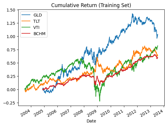
The benchmark's return is undoubtedly more stable than any of its constituents. TLT (bond) also has a smoother curve among the others, but the negative relationship with VTI (equity) is obvious too. By averaging them up, the benchmark yields better risk-adjusted return. However, the performance is still not as good as expected (1.0). There may be several reasons for the unsatisfying Sharpe:
Sampling error. Since GLD is founded at the end of 2004, the test of the portfolio is conducted on the 8-year data set of 2005-2013. Compared to the 30-year statistics provided by Lazy Portfolio ETF, statistical error may occur.
Partial portfolio. The constructed portfolio only consists of equity, long-term bond, and gold, while Ray Dalio's All Weather Portfolio also includes intermediate-term bonds and other commodities. It's only a "some weather" portfolio. Some risks aren't hedged away yet (e.g. yield curve inversion).
Use of daily returns. The tested volatility is 9.13%, significantly higher than Lazy Portfolio ETF's 7.21%. That may be caused by using different time frames for calculations. Assuming daily rebalancing may increase the volatility. As volatility is mean-reverting, daily volatility is usually higher than the longer time frame (e.g. monthly, yearly).
Anyway, as long as the calculation is consistent, the benchmark and the trading systems are still comparable.
The next article is about choosing trading rules and variations.


